A Gentle Introduction to Graph Neural Networks 学习笔记

Neural networks have been adapted to leverage (lever:杠杆，leverage:借助) the structure and properties of graphs. We explore the components needed for building a graph neural network - and motivate the design choices behind them.

Understanding Convolutions on Graphs

social networks
molecules
organizations
citations
physical models
transactions（交易）

$\Rightarrow$ Graphs

Neural Networks(NNs): fixed-size and/or regular-structured inputs

Graph Neural Networks(GNNs): operate naturally on graph-structured data

The Challenges of Computation on Graphs

Lack of Consistent Structure (but flexible)
Node-Order Equivariance(等效性)
Scalability $n \sim m$ Sparse

Problem Setting and Notation

Node Classification: Classifying individual
Graph Classification: Classifying entire graphs.
Node Clustering: Grouping together similar nodes based on connectivity.
Link Prediction: Predicting missing links.
Influence Maximization: Identifying influential nodes.

Polynomial Filters on Graphs

Basic Concepts

We consider simple graphs (no multiple edges or loops),

\mathcal{G}=\{\mathcal{V}, \mathcal{E}\}

$\mathcal{V}(\mathcal{G})=\left\{v_1, \ldots, v_n\right\}$ is called the vertex set with $n=|\mathcal{V}|$ ;
$\mathcal{E}(\mathcal{G})=\left\{e_{i j}\right\}$ is called the edge set with $m=|\mathcal{E}|$ ;
An edge $e_{i j}$ connects vertices $v_i$ and $v_j$ if they are adjacent or neighbors. One possible notation for adjacency is $v_i \sim v_j$ ;
The number of neighbors of a node $v$ is called the degree of $v$ and is denoted by $d(v), d\left(v_i\right)=\sum_{v_i \sim v_j} e_{i j}$ . If all the nodes of a graph have the same degree, the graph is regular (正则图); The nodes of an Eulerian graph have even degree.
A graph is complete if there is an edge between every pair of vertices.
$\mathcal{H}$ is a subgraph of $\mathcal{G}$ if $\mathcal{V}(\mathcal{H}) \subseteq \mathcal{V}(\mathcal{G})$ and $\mathcal{E}(\mathcal{H}) \subseteq \mathcal{E}(\mathcal{G})$ ;
a subgraph $\mathcal{H}$ is an induced subgraph of $\mathcal{G}$ if two vertices of $\mathcal{V}(\mathcal{H})$ are adjacent if and only if they are adjacent in $\mathcal{G}$ .
A clique is a complete subgraph of a graph.
A path of $k$ vertices is a sequence of $k$ distinct vertices such that consecutive vertices are adjacent.
A cycle is a connected subgraph where every vertex has exactly two neighbors.
A graph containing no cycles is a forest. A connected forest is a tree.
A graph is called k-partite if its set of vertices admits a partition into $k$ classes such that the vertices of the same class are not adjacent.
bipartite 二部图

Adjacency Matrix

For a graph with $n$ vertices, the entries of the $n \times n$ adjacency matrix are defined by:
$\begin{gathered} \mathbf{A}:= \begin{cases}A_{i j}=1 & \text { if there is an edge } e_{i j} \\ A_{i j}=0 & \text { if there is no edge } \\ A_{i i}=0\end{cases} \\ \mathbf{A}=\left[\begin{array}{llll} 0 & 1 & 1 & 0 \\ 1 & 0 & 1 & 1 \\ 1 & 1 & 0 & 0 \\ 0 & 1 & 0 & 0 \end{array}\right] \end{gathered}$
$\mathbf{A}$ is a real-symmetric matrix: it has $n$ real eigenvalues and its $n$ real eigenvectors form an orthonormal basis.
Let $\left\{\lambda_1, \ldots, \lambda_i, \ldots, \lambda_r\right\}$ be the set of distinct eigenvalues. The eigenspace $S_i$ contains the eigenvectors associated with $\lambda_i$
$S_i=\left\{\boldsymbol{x} \in \mathbb{R}^n \mid \mathbf{A} \boldsymbol{x}=\lambda_i \boldsymbol{x}\right\}$
For real-symmetric matrices, the algebraic multiplicity is equal to the geometric multiplicity, for all the eigenvalues.
The dimension of $S_i$ (geometric multiplicity) is equal to the multiplicity of $\lambda_i$ . 代数重数和几何重数。
If $\lambda_i \neq \lambda_j$ then $S_i$ and $S_j$ are mutually orthogonal. 相互正交
We consider real-valued functions on the set of the graph’s vertices, $\boldsymbol f: \mathcal V \to \R$ . Such a function assigns a real number to each graph node. 规定点权
$f$ is a vector indexed by the graph’s vertices, hence $f \in \mathbb{R}^n$ . $n$ 个节点对应 $n$ 个点权。
Notation: $f=\left(f\left(v_1\right), \ldots, f\left(v_n\right)\right)=(f(1), \ldots, f(n))$ . 记号
The eigenvectors of the adjacency matrix, $\mathbf{A} \boldsymbol{x}=\lambda \boldsymbol{x}$ , can be viewed as eigenfunctions. 特征函数
The adjacency matrix can be viewed as an operator（作用是将一个节点的权值变为相邻节点的权值）

\boldsymbol{g}=\mathbf{A} \boldsymbol{f} ; g(i)=\sum_{i \sim j} f(j)

It can also be viewed as a quadratic form（二次型）: 作用是对于每一条边，计算相邻节点的权值之和。

\boldsymbol{f}^{\top} \mathbf{A} \boldsymbol{f}=\sum_{e_{i j}} f(i) f(j)

Incidence Matrix

Let each edge in the graph have an arbitrary but fixed orientation;
The incidence matrix of a graph is a $|\mathcal{E}| \times|\mathcal{V}|(m \times n)$ matrix defined as follows:（关联矩阵）

\begin{aligned} & \nabla:= \begin{cases}\nabla_{e v}=-1 & \text { if } v \text { is the initial vertex of edge } e \\ \nabla_{e v}=1 & \text { if } v \text { is the terminal vertex of edge } e \\ \nabla_{e v}=0 & \text { if } v \text { is not in } e\end{cases} \\ & \nabla=\left[\begin{array}{cccc} -1 & 1 & 0 & 0 \\ 1 & 0 & -1 & 0 \\ 0 & -1 & 1 & 0 \\ 0 & -1 & 0 & +1 \end{array}\right] \end{aligned}

关联矩阵是离散微分算子。

Laplacian Matrix

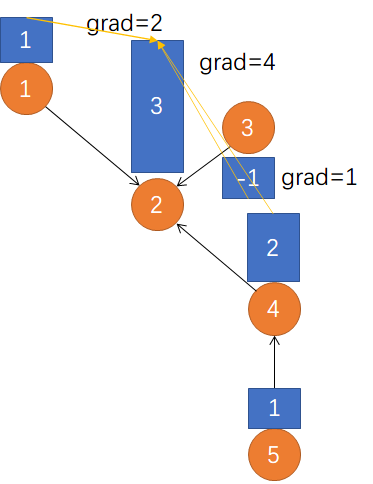
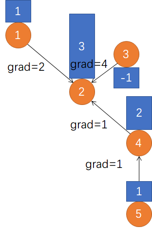
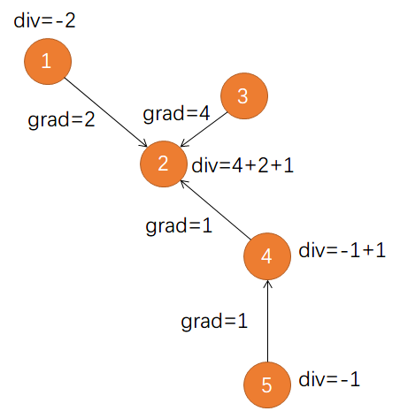
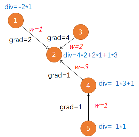
对应连续情况梯度+散度。

$\mathbf{L}=\nabla^{\top} \nabla$
$(\mathbf{L} \boldsymbol{f})\left(v_i\right)=\sum_{v_j \sim v_i}\left(f\left(v_i\right)-f\left(v_j\right)\right)$
其中 $\mathbf{L} \boldsymbol{f}$ 是一个新的函数。
Connection between the Laplacian and the adjacency matrices:

\mathbf{L}=\mathbf{D}-\mathbf{A}

The degree matrix: $\mathbf{D}:=D_{i i}=d\left(v_i\right)$ . Eigen Value 0: Correspond to $\bold{1}_n$ . In degree=Out degree

\mathbf{L}=\left[\begin{array}{cccc} 2 & -1 & -1 & 0 \\ -1 & 3 & -1 & -1 \\ -1 & -1 & 2 & 0 \\ 0 & -1 & 0 & 1 \end{array}\right]

The Laplacian matrix of an undirected weighted graph

We consider undirected weighted graphs: Each edge $e_{i j}$ is weighted by $w_{i j}>0$ .
The Laplacian as an operator:

(\mathbf{L} \boldsymbol{f})\left(v_i\right)=\sum_{v_j \sim v_i} w_{i j}\left(f\left(v_i\right)-f\left(v_j\right)\right)

As a quadratic form:

\boldsymbol{f}^{\top} \mathbf{L} \boldsymbol{f}=\frac{1}{2} \sum_{e_{i j}} w_{i j}\left(f\left(v_i\right)-f\left(v_j\right)\right)^2

$\mathbf{L}$ is symmetric and positive semi-definite.
L has $n$ non-negative, real-valued eigenvalues:

0=\lambda_1 \leq \lambda_2 \leq \ldots \leq \lambda_n \text {. }

我是这么想的，先对整张图进行统计，计算一条边在所有或部分 $(u,v)$ 点对之间最短路路径的出现次数。设定一定阈值，在阈值以上的边称为主干道，主干道的点称为主节点。从开始节点到结束节点，可以抽象为从开始节点到主节点，主节点之间移动，从主节点到结束节点。因此，算法可以分为：

预处理主节点之间的最短路
通过Dijkstra算法得到离当前开始节点最近的主节点，离结束节点最近的主节点（这个时候可能要把边反向）
通过预处理的最短路计算主节点之间的距离

后面发现和 CCH 算法类似