Terminologies
homogeneity 齐次性。
Thevenin’s theorem, Norton’s theorem. 戴维宁定律 诺顿定律。
Kirchhoff’s laws are used to analyze a circuit without changing its original configuration, but tedious computations involved in case of complex circuits.
Thevenin’s and Norton’s theorems are used to analyze complex circuit by simplifying its configuration.
核心在于简化电路。
Linearity Property
Linear relationship between cause and effect ( and ).
Only applying to resistors.
homogeneity property and additivity property.
- if , then .
- if , then .
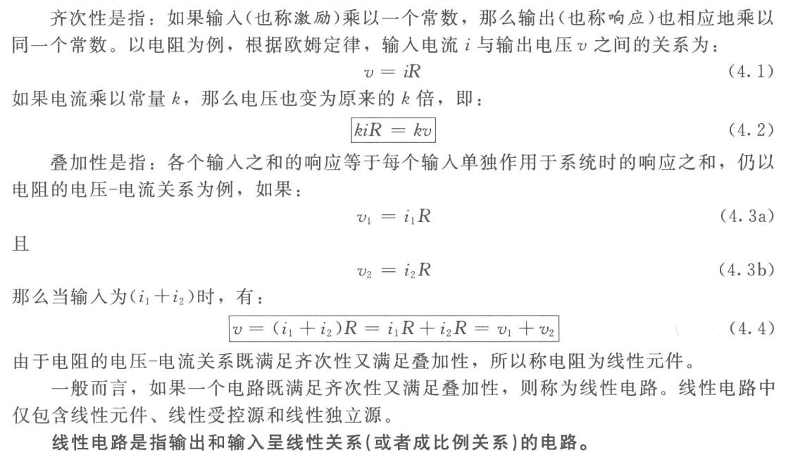
All elements are linear $\Rightarrow $ circuit is linear.

.
Power is nonlineraly related to voltage or current.
Equivalent resistance can be found by linearity.
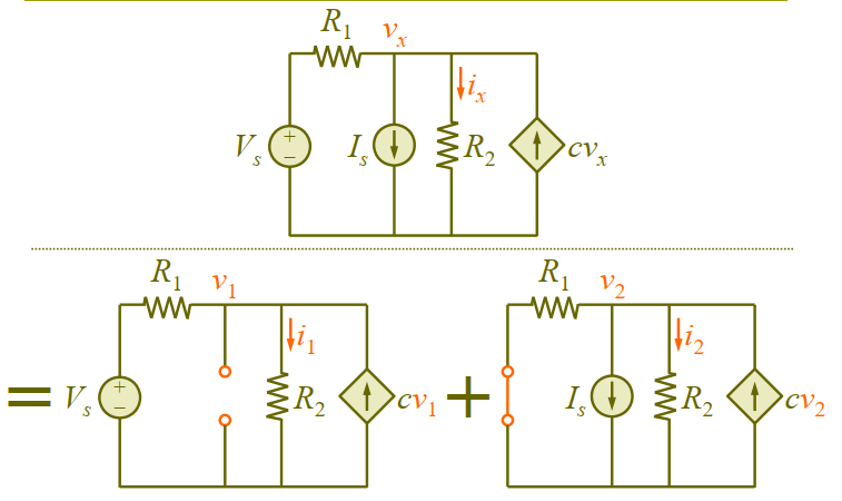
Superposition principle
It relies on linearity property and states that voltage across (or current through) an element in a linear circuit is algebraic sum of voltages across (or currents through) that element due to each independent source acting alone.
功率不符合叠加原理。
Pros and cons of superposition
- Reducing complex circuit to simpler one by
- Replacing voltage source by short circuit.
- Replacing current source by open circuit.
- Involving more calculation of analyzing contributions due to each source.
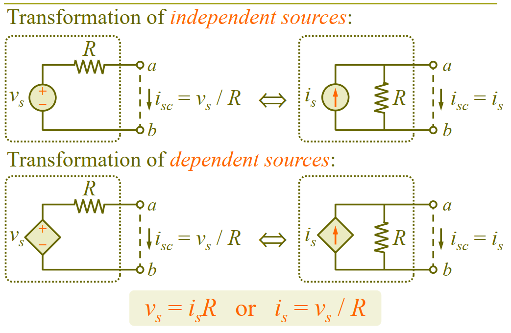
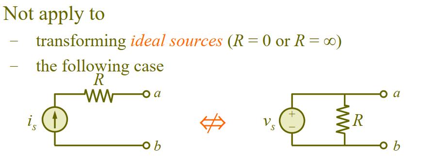
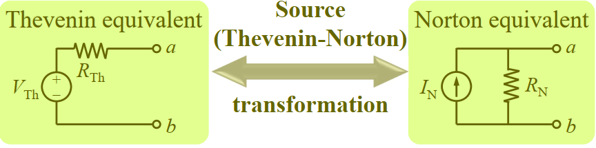
Source transformation.
- Tools for simplifying circuits: series parallel combination, or transformation, source transformation.
- Basic idea: equivalence.
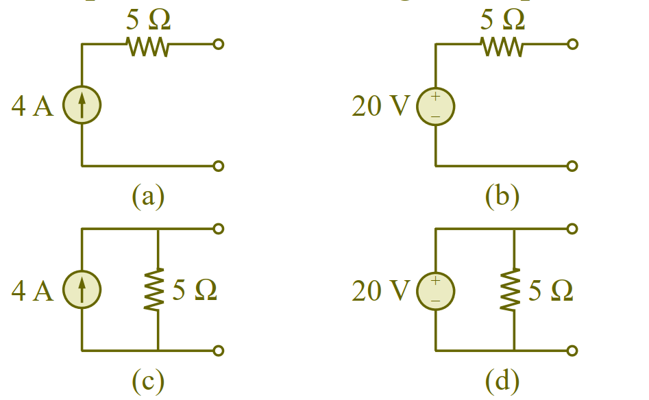
Replace a voltage source in series with a resistor by a current source in parallel with a resistor. or vice versa.
Active Sign Convention.
, 。
电池的内阻。
第一眼进行化简:
parallel with 4 ohm.
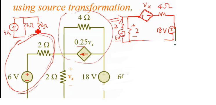
Transform to current source.
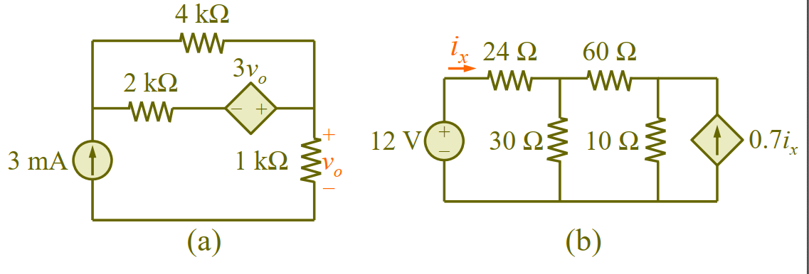
3mA * 1k Ohm
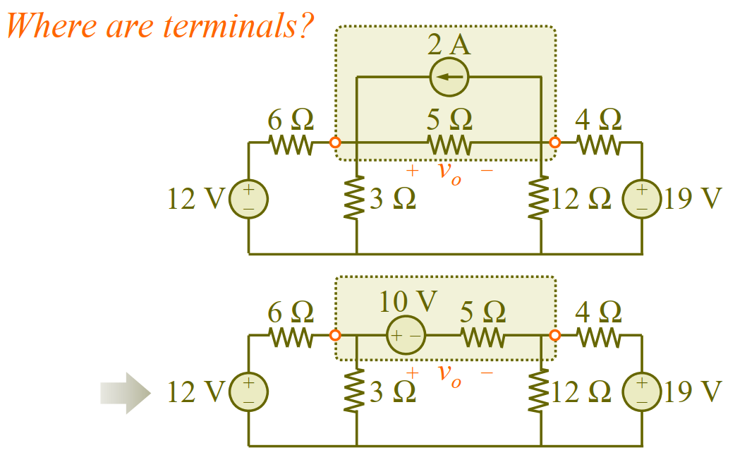
Where is ?
回避改变未知量。
适用条件:
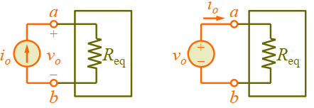
Thevenin’s Theroem
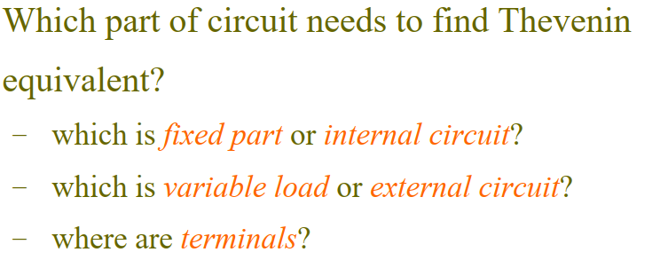
Any linear two-terminal circuit can be replaced by equivalent circuit.
为端口的开路电压, 为独立源关闭时端口的输入(或等效电阻)。
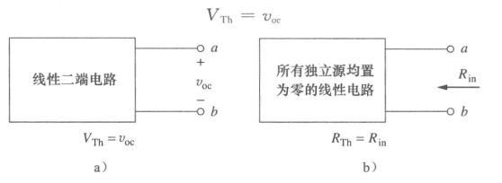
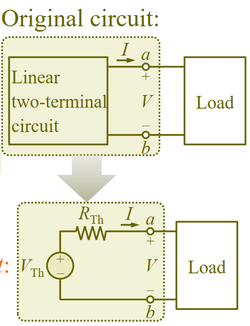
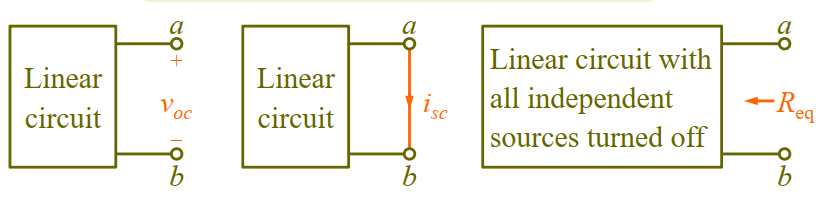
A linear two-terminal circuit can be replaced by an equivalent circuit consisting of a voltage sourse in series with a resistor , where is open-circuit voltage at terminals and is input or equivalent resistance at terminals when all independent sources are turned off.
Can be mathematically derived.
is open-circuit voltage across two terminals of original circuit.
Independent sources are turned off. (电压源短路,电流源断路) To Find
Case 1: Without dependent sources.
Superposition.

Find Case 2: With dependent sources.
Obtain . Assume any for easier calculation.
No independent source .
Determine Thevenin resistance. Use symbol or one volt.
- Excited with current source + nodal analysis.
- Excited with voltage source + mesh analysis.
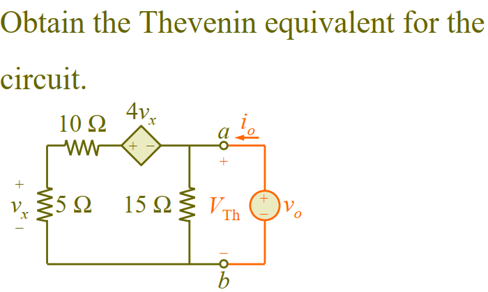
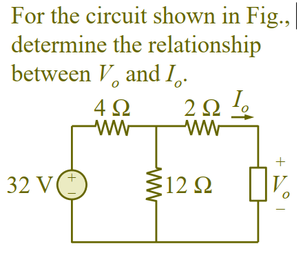
 $$
0.1i+\frac{20i-2v}{40}+i=\frac{v}{10} \Rightarrow v=i+5i-0.5v+10i\Rightarrow v=10i\\
i_o=0.1i+\frac{v}{10}=1.1i\\
v_o=20i+v=30i
$$
$$
0.1i+\frac{20i-2v}{40}+i=\frac{v}{10} \Rightarrow v=i+5i-0.5v+10i\Rightarrow v=10i\\
i_o=0.1i+\frac{v}{10}=1.1i\\
v_o=20i+v=30i
$$
Norton’s Theorem
Determine any two of the variables.
equals to independent source.
Standalone circuits.
The Wheatstone bridge. Not parellel. Balanced Bridge.
- Find or using basic laws, nodal analysis, mesh analysis, source transformation, linearity or superposition.
- Find or when dependent sources exist.
- Apply .
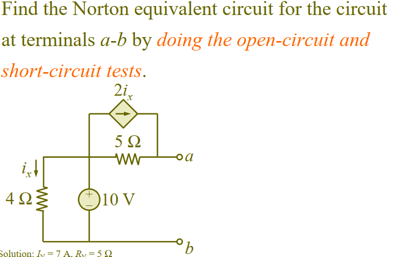
- Do open-circuit and short-circuit tests to original circuit and find .
- Find equivalent circuit that you are better at, and find the other one using source transformation.
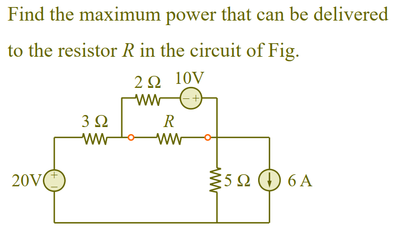
Power transferred to load
希望传递给负载的功率最大。需要注意,为负载传输最大功率会造成电路内部损耗大于或等于传输给负载的功率。
Find the first derivative: power with respect to .
Load branch.
- Maximum power problem.
- find Thevenin equivalent.
- Maximum power theorem.
- Difference between power supplied to load and loss
- maximum power minimum loss.
Problems
Chapter 4, Problem 1.

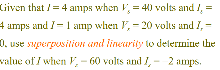
Linerity Properity.
Chapter 4, Problem 4.

Reverse Application of Linearity.
Chapter 4, Problem 5
Chapter 4, Problem 8.

Let , where and are due to 9-V and 3-V sources respectively. To find , consider the circuit below.

To find , consider the circuit below.

Chapter 4, Problem 11

Superposition with control sources.

At node a,
At node b,
But

Chapter 4, Problem 14.

Chapter 4, Problem 21.

可以合并并联电流源的电流,串联电压源的电压。
Chapter 4, Problem 23.

Chapter 4, Problem 24.


Chapter 4, Problem 33.
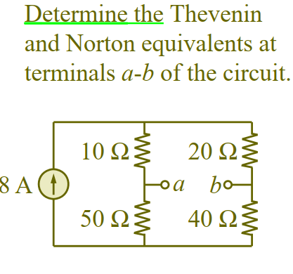
Determin and at terminals 1-2 of each of the circuits of Fig. 4.101.

a.
b. Use source transformation.
Chapter 4, Problem 34.

For , turn voltage source into short circuit and current source into open circuit like this,

For , use nodal analysis.

认为只是使用电压表测量两点电压,因此这个branch没有电流。
At node 1,
At node 2, (no current)
另外,可以考虑是 standalone circuit, 直接电压叠加。
Chapter 4, Problem 36.


Chapter 4, Problem 37.

So there is short circuit.
Chapter 4, Problem 39.

Chapter 4, Problem 40.

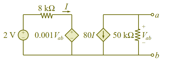
Thevenin Equvalent with dependent source.
To obtain , we apply KVL to the loop,
To find , we remove the independent source 70-V and apply a 1-V source at terminals a-b, as shown in the circuit below.

We notice that .
Chapter 4, Problem 42.


We can also see that there will be no current across the middle branch.

Easier with mesh analysis.
Chapter 4, Problem 44.


Chapter 4, Problem 47.
Chapter 4, Problem 49.

Chapter 4, Problem 53.

Dependent Source.


Chapter 4, Problem 54.


注意三点,第一点是关掉 3V,第二点Mesh Analysis关掉独立源,第三点电阻可能是负数。
使用Mesh Analysis,对应电路上的电压、电流,需要注意支路电流的表达式。
Chapter 4, Problem 59.

Chapter 4, Problem 64

